OLS

Typically when we use linear regression (or OLS) to model things in social science, we care about the coefficients so that we can find marginal effects: what happens to the outcome when we move an explanatory variable up and down? Or in the case of categorical explanatory variables, what’s the average outcome across different categories?

Because of this, we don’t typically think about distributions or parameters when working with OLS. BUT WE CAN. And thinking about how outcome distributions change in response to explanatory variables opens up possibilities for modeling all sorts of speical non-normal outcomes.

library(tidyverse)
library(palmerpenguins)
library(marginaleffects)
library(patchwork)
library(parameters)
library(broom)
library(distributional)
library(ggdist)
library(brms)
library(tidybayes)

options(mc.cores = 4)  # Use 4 cores for {brms}

theme_set(theme_minimal())

penguins <- penguins |> drop_na(sex)

For instance, we can model the distribution of penguin weights:

ggplot(penguins, aes(x = body_mass_g)) +
  geom_density()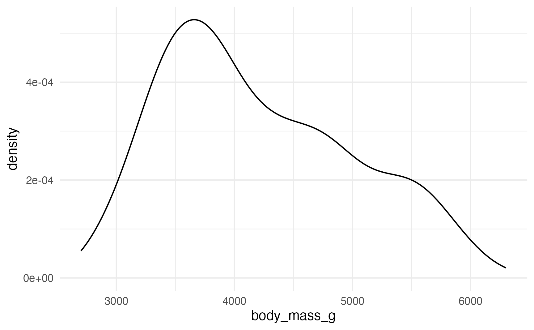

That doesn’t look very normal—it’s skewed right with a long tail. That’s likely because of other factors, like penguin species. Let’s color by species:

ggplot(penguins, aes(x = body_mass_g, color = species)) +
  geom_density()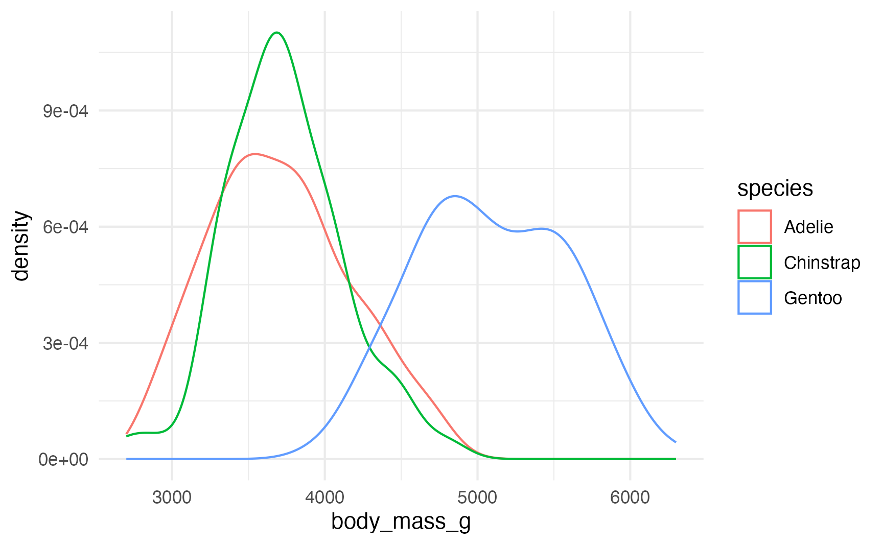

That original lumpy skewed distribution is actually the combination of three separate relatively-normal-looking distributions.

Let’s model body mass based on species:

model <- lm(body_mass_g ~ species, data = penguins)

# parameters::model_parameters() gives a nice summary of the coefficients
model_parameters(model)
## Parameter           | Coefficient |    SE |             95% CI | t(330) |      p
## --------------------------------------------------------------------------------
## (Intercept)         |     3706.16 | 38.14 | [3631.14, 3781.18] |  97.18 | < .001
## species [Chinstrap] |       26.92 | 67.65 | [-106.16,  160.01] |   0.40 | 0.691 
## species [Gentoo]    |     1386.27 | 56.91 | [1274.32, 1498.22] |  24.36 | < .001
## 
## Uncertainty intervals (equal-tailed) and p-values (two-tailed) computed
##   using a Wald t-distribution approximation.

# So does broom::tidy()
tidy(model, conf.int = TRUE)
## # A tibble: 3 × 7
##   term             estimate std.error statistic   p.value conf.low conf.high
##   <chr>               <dbl>     <dbl>     <dbl>     <dbl>    <dbl>     <dbl>
## 1 (Intercept)        3706.       38.1    97.2   6.88e-245    3631.     3781.
## 2 speciesChinstrap     26.9      67.7     0.398 6.91e-  1    -106.      160.
## 3 speciesGentoo      1386.       56.9    24.4   1.01e- 75    1274.     1498.

Since these are all in grams, we can interpret these coefficients directly (and we can think of them as sliders and switches)

It’s a little annoying to have all these estimates be based around Adelie. We can get around that in a couple ways:

Use marginaleffects::avg_predictions(), which deals with all the relative group averages automatically:

avg_predictions(model, variables = "species")
## 
##    species Estimate Std. Error     z Pr(>|z|)   S 2.5 % 97.5 %
##  Adelie        3706       38.1  97.2   <0.001 Inf  3631   3781
##  Gentoo        5092       42.2 120.6   <0.001 Inf  5010   5175
##  Chinstrap     3733       55.9  66.8   <0.001 Inf  3624   3843
## 
## Type:  response 
## Columns: species, estimate, std.error, statistic, p.value, s.value, conf.low, conf.high

Fit a model without the intercept using 0 +:

model_sans_intercept <- lm(body_mass_g ~ 0 + species, data = penguins)
tidy(model_sans_intercept, conf.int = TRUE)
## # A tibble: 3 × 7
##   term             estimate std.error statistic   p.value conf.low conf.high
##   <chr>               <dbl>     <dbl>     <dbl>     <dbl>    <dbl>     <dbl>
## 1 speciesAdelie       3706.      38.1      97.2 6.88e-245    3631.     3781.
## 2 speciesChinstrap    3733.      55.9      66.8 8.16e-194    3623.     3843.
## 3 speciesGentoo       5092.      42.2     121.  6.31e-275    5009.     5176.

These coefficients show us the averages for each species, or the \(\mu\) in a normal distribution:

species_averages <- avg_predictions(model, variables = "species")

ggplot(penguins, aes(x = body_mass_g, fill = species)) +
  stat_density(geom = "area", alpha = 0.6, position = position_identity()) +
  geom_vline(data = species_averages, aes(xintercept = estimate, color = species))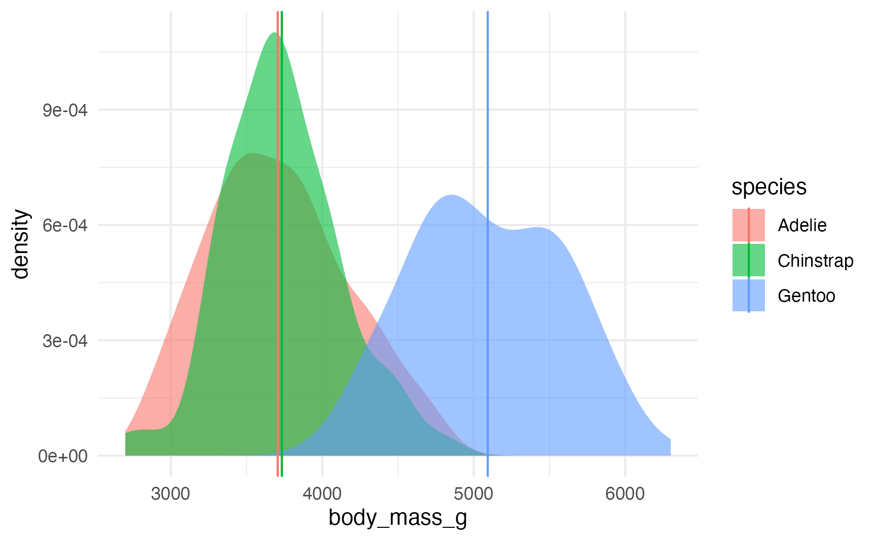

Getting closer to distributional regression

We’re halfway to describing the outcome using distributions—we just need to find the standard deviation for each group.

It’s tempting to use the standard error column in the model results, but that’s wrong! That’s the standard deviation of the coefficient, not the standard deviation for the group.

One way to use the model results to find group-specific distributional standard deviations is to find the standard deviation of the residuals. We can use broom::augment() to add the fitted values and residuals to each row in the original data:

fitted_values <- augment(model)
fitted_values
## # A tibble: 333 × 8
##    body_mass_g species .fitted .resid    .hat .sigma   .cooksd .std.resid
##          <int> <fct>     <dbl>  <dbl>   <dbl>  <dbl>     <dbl>      <dbl>
##  1        3750 Adelie    3706.   43.8 0.00685   461. 0.0000209     0.0955
##  2        3800 Adelie    3706.   93.8 0.00685   461. 0.0000960     0.204 
##  3        3250 Adelie    3706. -456.  0.00685   461. 0.00227      -0.993 
##  4        3450 Adelie    3706. -256.  0.00685   461. 0.000715     -0.558 
##  5        3650 Adelie    3706.  -56.2 0.00685   461. 0.0000344    -0.122 
##  6        3625 Adelie    3706.  -81.2 0.00685   461. 0.0000718    -0.177 
##  7        4675 Adelie    3706.  969.  0.00685   458. 0.0102        2.11  
##  8        3200 Adelie    3706. -506.  0.00685   461. 0.00279      -1.10  
##  9        3800 Adelie    3706.   93.8 0.00685   461. 0.0000960     0.204 
## 10        4400 Adelie    3706.  694.  0.00685   460. 0.00525       1.51  
## # ℹ 323 more rows

We can then find the standard deviation of the .resid column:

penguin_parameters <- fitted_values |> 
  group_by(species) |> 
  summarize(mu = mean(.fitted), sigma = sd(.resid))
penguin_parameters
## # A tibble: 3 × 3
##   species      mu sigma
##   <fct>     <dbl> <dbl>
## 1 Adelie    3706.  459.
## 2 Chinstrap 3733.  384.
## 3 Gentoo    5092.  501.

These values represent the \(\mu\) and \(\sigma\) for each of the species distributions. We can confirm it with a plot:

ggplot(penguins, aes(x = body_mass_g, fill = species)) +
  stat_density(geom = "area", alpha = 0.6, position = position_identity()) +
  stat_function(data = penguin_parameters, aes(x = NULL, y = NULL, color = species[1]),
                fun = function(x, mu, sigma) dnorm(x, mean = mu, sd = sigma),
                args = list(mu = penguin_parameters$mu[1], sigma = penguin_parameters$sigma[1]), size = 1) +
  stat_function(data = penguin_parameters, aes(x = NULL, y = NULL, color = species[2]),
                fun = function(x, mu, sigma) dnorm(x, mean = mu, sd = sigma),
                args = list(mu = penguin_parameters$mu[2], sigma = penguin_parameters$sigma[2]), size = 1) +
  stat_function(data = penguin_parameters, aes(x = NULL, y = NULL, color = species[3]),
                fun = function(x, mu, sigma) dnorm(x, mean = mu, sd = sigma),
                args = list(mu = penguin_parameters$mu[3], sigma = penguin_parameters$sigma[3]), size = 1)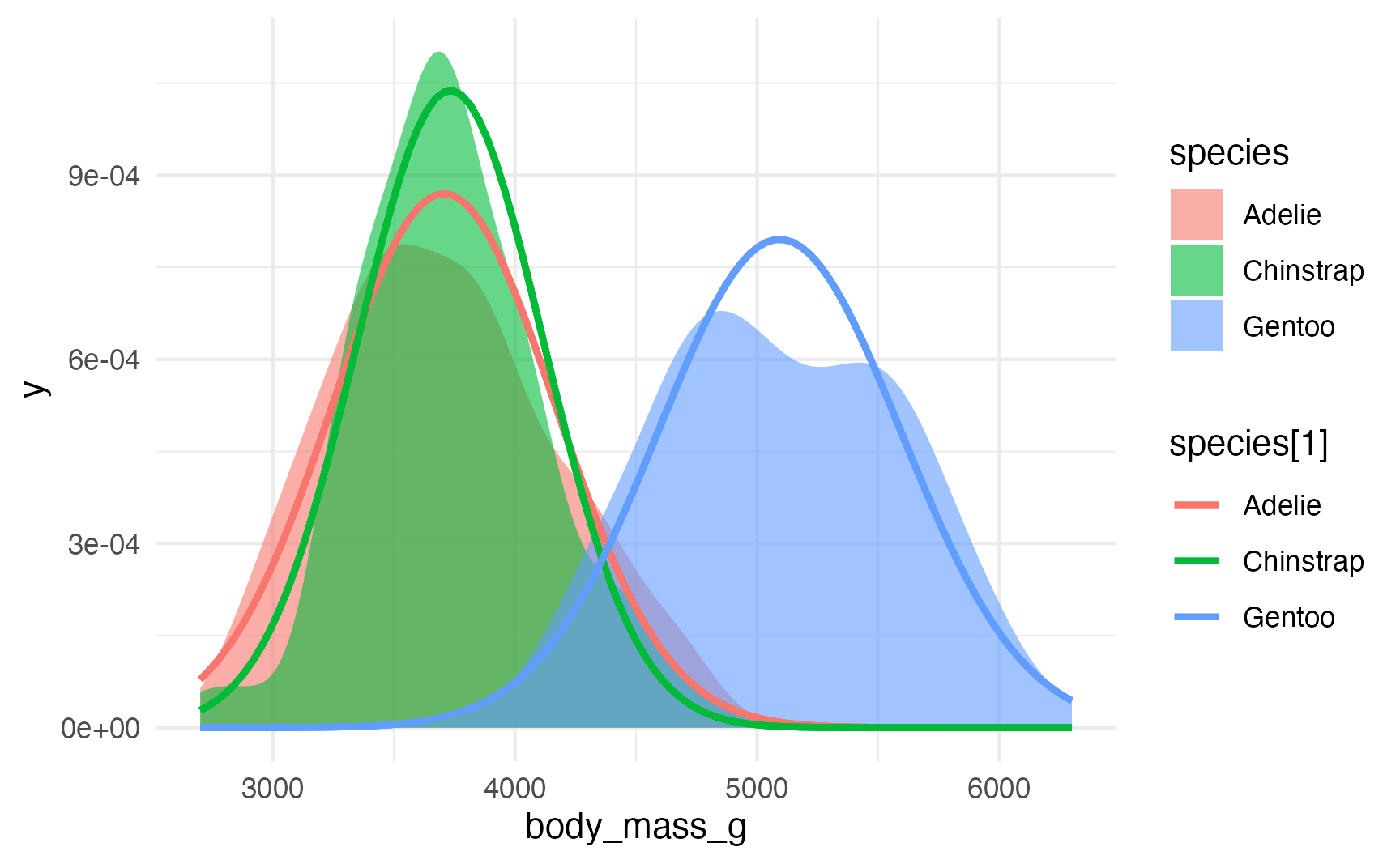

↑ That’s all super gross code though. Instead of adding stat_function() layers manually like that, we can use the {distributional} R package, which lets you work with distribution objects:

penguin_parameters_dist <- penguin_parameters |> 
  mutate(dist = dist_normal(mu = mu, sigma = sigma))
penguin_parameters_dist
## # A tibble: 3 × 4
##   species      mu sigma
##   <fct>     <dbl> <dbl>
## 1 Adelie    3706.  459.
## 2 Chinstrap 3733.  384.
## 3 Gentoo    5092.  501.
## # ℹ 1 more variable: dist <dist>

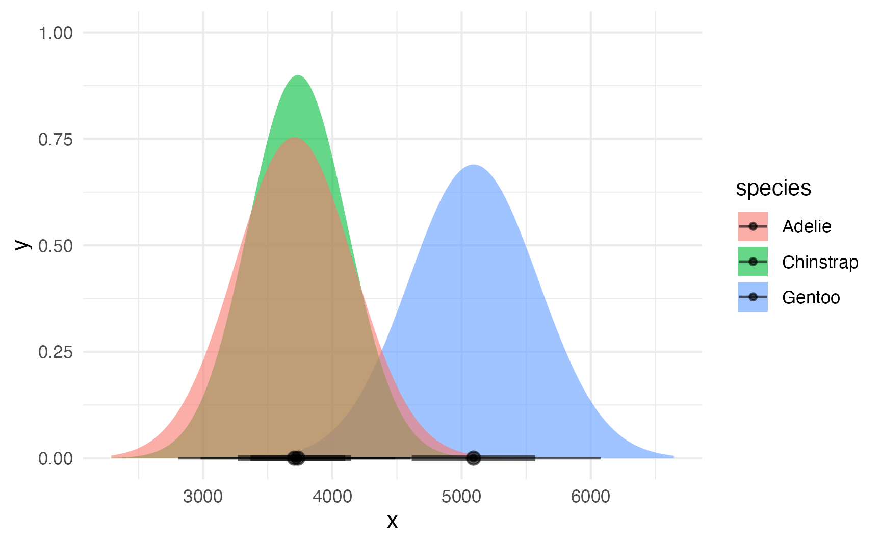
Plotting this is much easier with the {ggdist} package:

ggplot() +
  stat_slabinterval(
    data = penguin_parameters_dist,
    aes(dist = dist, fill = species, y = 0),
    alpha = 0.6
  )

We can even combine these estimated density plots with the actual data densities with some minor tweaks to the function arguments (and adjusting the y-axis range):

ggplot(penguins, aes(x = body_mass_g, color = species)) +
  stat_density(geom = "line", position = position_identity()) +
  stat_slabinterval(
    data = penguin_parameters_dist,
    aes(dist = dist, fill = species, y = 0),
    alpha = 0.4, normalize = "none", inherit.aes = FALSE
  ) +
  coord_cartesian(ylim = c(0, 0.0011))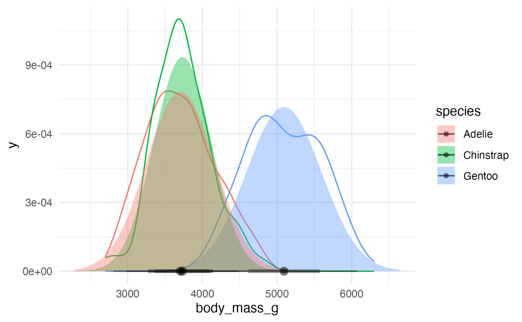

Explicit distributional regression with Bayesianism

It’s neat that we can get the \(\mu\) and \(\sigma\) out of a regular OLS regression model and think about the outcomes as distributions. We can also use continuous predictors to show how the \(\mu\) and \(\sigma\) change across different values of those predictors, but getting that information out of the results of lm() requires a bunch of work.

Fortunately, Bayesian regression (with the magical {brms} package) lets us explicitly model both the \(\mu\) and—optionally—the \(\sigma\).

\[ \begin{aligned} \text{Penguin weight}_i &\sim \mathcal{N}(\mu_i, \sigma_i) \\ \mu_i &= \beta_0 + \beta_{1 \dots 2}\ \text{Species}_i \end{aligned} \]

model_bayes <- brm(
  bf(body_mass_g ~ species),
  data = penguins,
  family = gaussian,
  chains = 4, iter = 2000, seed = 1234,
  file = "models/model_ols_bayes", refresh = 0
)
model_bayes
##  Family: gaussian 
##   Links: mu = identity; sigma = identity 
## Formula: body_mass_g ~ species 
##    Data: penguins (Number of observations: 333) 
##   Draws: 4 chains, each with iter = 2000; warmup = 1000; thin = 1;
##          total post-warmup draws = 4000
## 
## Regression Coefficients:
##                  Estimate Est.Error l-95% CI u-95% CI Rhat Bulk_ESS Tail_ESS
## Intercept         3705.19     37.72  3631.14  3780.04 1.00     3455     2930
## speciesChinstrap    30.28     67.42  -104.26   158.56 1.00     3506     2919
## speciesGentoo     1387.41     58.25  1273.82  1504.04 1.00     3777     2992
## 
## Further Distributional Parameters:
##       Estimate Est.Error l-95% CI u-95% CI Rhat Bulk_ESS Tail_ESS
## sigma   462.16     18.03   428.23   498.85 1.00     3853     3221
## 
## Draws were sampled using sampling(NUTS). For each parameter, Bulk_ESS
## and Tail_ESS are effective sample size measures, and Rhat is the potential
## scale reduction factor on split chains (at convergence, Rhat = 1).

model_parameters(model_bayes, verbose = FALSE)
## # Fixed Effects
## 
## Parameter        |  Median |             95% CI |     pd |  Rhat |     ESS
## --------------------------------------------------------------------------
## (Intercept)      | 3704.87 | [3631.14, 3780.04] |   100% | 1.000 | 3434.00
## speciesChinstrap |   31.75 | [-104.26,  158.56] | 67.07% | 1.000 | 3485.00
## speciesGentoo    | 1387.17 | [1273.82, 1504.04] |   100% | 0.999 | 3774.00
## 
## # Sigma
## 
## Parameter | Median |           95% CI |   pd |  Rhat |     ESS
## --------------------------------------------------------------
## sigma     | 461.66 | [428.23, 498.85] | 100% | 1.001 | 3814.00

model_bayes |> 
  gather_draws(`^b_.*`, regex = TRUE) |>
  ggplot(aes(x = .value, fill = .variable)) +
  stat_halfeye(normalize = "xy") +
  labs(x = "Coefficient value", y = NULL) +
  facet_wrap(vars(.variable), scales = "free_x") +
  guides(fill = "none") +
  theme(axis.text.y = element_blank())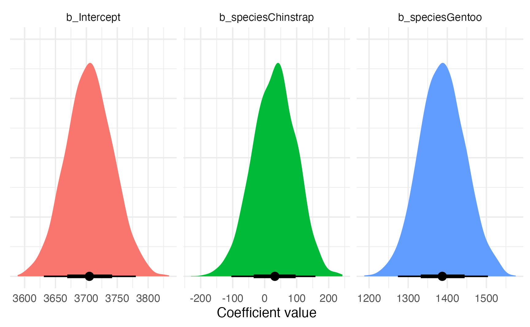

plot_predictions_equal_variances <- model_bayes |> 
  avg_predictions(variables = "species") |> 
  posterior_draws() |> 
  ggplot(aes(x = draw, fill = species)) +
  stat_halfeye(normalize = "xy") +
  labs(x = "Predicted value", y = NULL) +
  facet_wrap(vars(species), scales = "free_x") +
  guides(fill = "none") +
  theme(axis.text.y = element_blank())
plot_predictions_equal_variances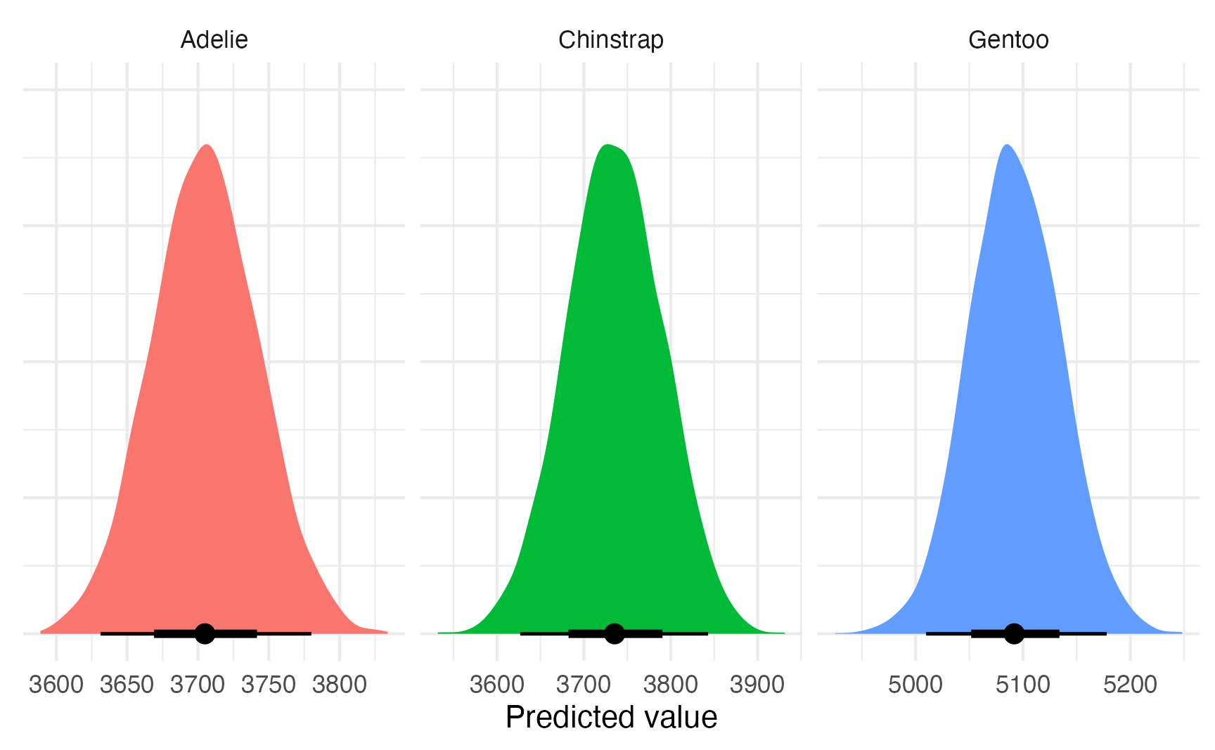

We can also explicitly model the \(\sigma\) part of the outcome, and we can even model it differently from the \(\mu\) part if we have reason to believe the process might be different. For simplicitly, we’ll just use the same explanatory variables for both parts:

\[ \begin{aligned} \text{Penguin weight}_i &\sim \mathcal{N}(\mu_i, \sigma_i) \\ \mu_i &= \beta_0 + \beta_{1 \dots 2}\ \text{Species}_i \\ \log(\sigma_i) &= \gamma_0 + \gamma_{1 \dots 2}\ \text{Species}_i \end{aligned} \]

model_bayes_sigma <- brm(
  bf(
    body_mass_g ~ species,
    sigma ~ 0 + species
  ),
  data = penguins,
  family = gaussian,
  chains = 4, iter = 2000, seed = 1234,
  file = "models/model_ols_sigma_bayes", refresh = 0
)
model_bayes_sigma
##  Family: gaussian 
##   Links: mu = identity; sigma = log 
## Formula: body_mass_g ~ species 
##          sigma ~ 0 + species
##    Data: penguins (Number of observations: 333) 
##   Draws: 4 chains, each with iter = 2000; warmup = 1000; thin = 1;
##          total post-warmup draws = 4000
## 
## Regression Coefficients:
##                        Estimate Est.Error l-95% CI u-95% CI Rhat Bulk_ESS
## Intercept               3706.19     37.83  3633.52  3780.70 1.00     4935
## speciesChinstrap          26.77     60.10   -89.23   147.82 1.00     4926
## speciesGentoo           1386.56     59.41  1274.78  1501.10 1.00     4735
## sigma_speciesAdelie        6.13      0.06     6.02     6.25 1.00     5642
## sigma_speciesChinstrap     5.96      0.09     5.79     6.14 1.00     4898
## sigma_speciesGentoo        6.22      0.06     6.10     6.35 1.00     5747
##                        Tail_ESS
## Intercept                  3182
## speciesChinstrap           3354
## speciesGentoo              3154
## sigma_speciesAdelie        3212
## sigma_speciesChinstrap     3054
## sigma_speciesGentoo        3546
## 
## Draws were sampled using sampling(NUTS). For each parameter, Bulk_ESS
## and Tail_ESS are effective sample size measures, and Rhat is the potential
## scale reduction factor on split chains (at convergence, Rhat = 1).

model_parameters(model_bayes_sigma, verbose = FALSE)
## # Fixed Effects
## 
## Parameter              |  Median |             95% CI |     pd |  Rhat |     ESS
## --------------------------------------------------------------------------------
## (Intercept)            | 3705.86 | [3633.52, 3780.70] |   100% | 1.001 | 4903.00
## speciesChinstrap       |   25.79 | [ -89.23,  147.82] | 66.77% | 1.000 | 4867.00
## speciesGentoo          | 1385.96 | [1274.78, 1501.10] |   100% | 1.000 | 4731.00
## sigma_speciesAdelie    |    6.13 | [   6.02,    6.25] |   100% | 1.000 | 5667.00
## sigma_speciesChinstrap |    5.96 | [   5.79,    6.14] |   100% | 1.000 | 4805.00
## sigma_speciesGentoo    |    6.22 | [   6.10,    6.35] |   100% | 1.000 | 5670.00

Now we have model parameters for the regular coefficients and the sigmas (prefixed with sigma_). For whatever reason, Stan works with these on the log scale, which is why they all look really tiny. We can unlog them by exponentiating them:

model_parameters(
  model_bayes_sigma, 
  keep = "sigma_",
  exponentiate = TRUE, 
  verbose = FALSE
)
## # Fixed Effects
## 
## Parameter              | Median |           95% CI |   pd |  Rhat |     ESS
## ---------------------------------------------------------------------------
## sigma_speciesAdelie    | 460.06 | [412.32, 517.71] | 100% | 1.000 | 5667.00
## sigma_speciesChinstrap | 385.97 | [326.90, 464.30] | 100% | 1.000 | 4805.00
## sigma_speciesGentoo    | 502.30 | [444.81, 573.58] | 100% | 1.000 | 5670.00

They’re the same as what we found earlier by calculating the standard deviation of the residuals!

penguin_parameters
## # A tibble: 3 × 3
##   species      mu sigma
##   <fct>     <dbl> <dbl>
## 1 Adelie    3706.  459.
## 2 Chinstrap 3733.  384.
## 3 Gentoo    5092.  501.

plot_predictions_different_variances <- model_bayes_sigma |> 
  avg_predictions(variables = "species") |> 
  posterior_draws() |> 
  ggplot(aes(x = draw, fill = species)) +
  stat_halfeye(normalize = "xy") +
  labs(x = "Predicted value", y = NULL) +
  facet_wrap(vars(species), scales = "free_x") +
  guides(fill = "none") +
  theme(axis.text.y = element_blank())
plot_predictions_different_variances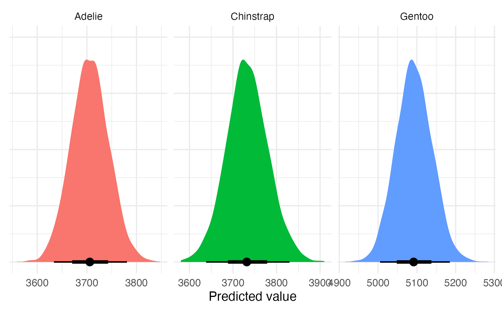

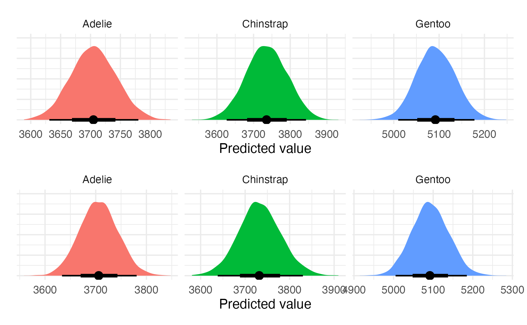
(plot_predictions_equal_variances + labs("Same sigma")) /
  (plot_predictions_different_variances + labs("Different sigmas"))