The Beta distribution represents a proportion between 0 and 1, but does not include 0 or 1. Zero/one-inflated Beta regression models separate processes for the 0s and 1s
Code
knitr::opts_chunk$set(fig.align ="center", fig.retina =3)library(tidyverse)library(marginaleffects)library(brms)library(tidybayes)library(parameters)library(tinytable)library(patchwork)library(extraDistr)library(ggridges)library(scales)library(betareg)# Data via the WHO via Kaggle# https://www.kaggle.com/datasets/lsind18/who-immunization-coveragetetanus <-readRDS("data/tetanus_pab.rds")tetanus_2020 <- tetanus |>filter(year ==2020) |># Cheat a littlemutate(prop_pab =ifelse(prop_pab >=0.97, 1, prop_pab)) |># Reverse thismutate(prop_unvacc =1- prop_pab)theme_set(theme_minimal())options(digits =3, width =120,tinytable_tt_digits =2)
Distribution intuition
The Beta distribution is great for proportions, but it doesn’t work with values that are exactly 0 or 1.
To get around this, we can use a special zero-inflated Beta regression. We’ll still model the \(\mu\) (mu) and \(\phi\) (phi) (or mean and precision) of the beta distribution, but we’ll also model one new special parameter \(\pi\) (pi; not 3.14, though). With zero-inflated regression, we’re actually modelling a mixture of data-generating processes:
A logistic regression model that predicts if an outcome is 0 or not, defined by \(\pi\)
A Beta regression model that predicts if an outcome is between 0 and 1 if it’s not zero, defined by \(\mu\) and \(\phi\)
Example: Modeling the proprotion of tetanus non-vaccinations
To illustrate this, we’ll look at 2020 PAB tetanus vaccination rates, since far more countries have reached or are approaching universal coverage. We’ll also cheat a little, since only 3 countries are actually at 100%—for the sake of this example, if a country is at 97% or more, we’ll consider that 100%.
Also, we’ll look at the reverse of the proportion, or the proportion of unvaccinated, since there is no one-inflated regression built into {brms}. Their suggestion is to either flip the value (like we’re doing here) or use zero-one-inflated regression and tell the zero-focused process there to be constant. Flipping the value is easier, so we’ll do that.
Let’s first see how many 0s we’re working with:
Code
tetanus_2020 |>count(prop_unvacc ==0) |>mutate(prop = n /sum(n))
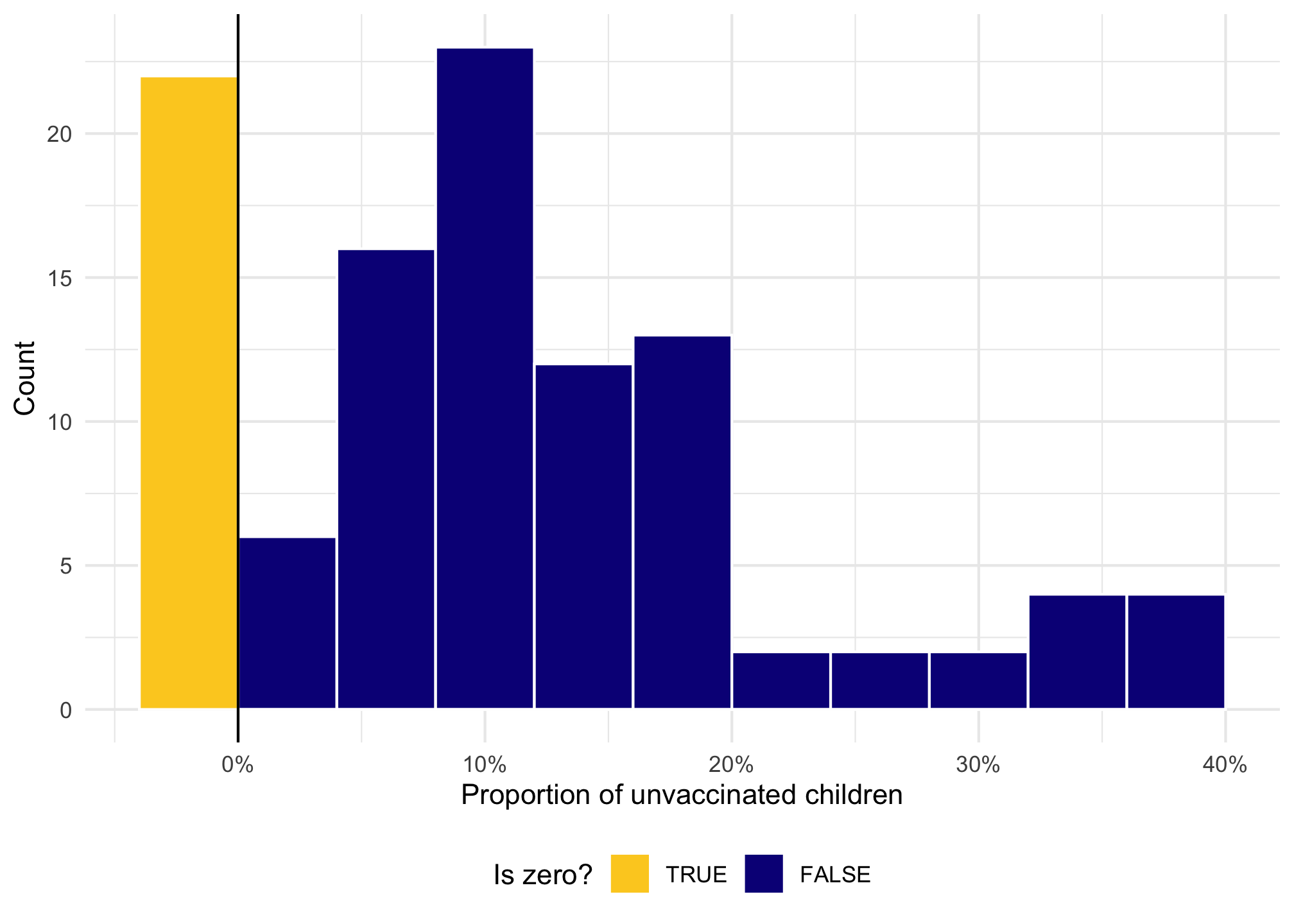
20% of the countries are fully vaccinated here (or have 0% unvaccinated kids). The 80% of countries with some unvaccinated children still follows a Beta distribution:
Code
tetanus_2020 |>mutate(is_zero = prop_unvacc ==0) |>mutate(prop_unvacc =ifelse(is_zero, -0.01, prop_unvacc)) |>ggplot(aes(x = prop_unvacc, fill = is_zero)) +geom_histogram(binwidth =0.04, boundary =0, color ="white") +geom_vline(xintercept =0) +scale_x_continuous(labels =label_percent()) +scale_fill_viridis_d(option ="plasma", end =0.9,guide =guide_legend(reverse =TRUE) ) +labs(x ="Proportion of unvaccinated children", y ="Count", fill ="Is zero?" ) +theme(legend.position ="bottom")
The only difference between regular Beta regression and zero-inflated Beta regression is that we have to specify one more parameter: zi. This corresponds to the \(\pi\) parameter and determines the zero/not-zero process.
To help with the intuition, we’ll first run a model where we don’t actually define a model for zi—it’ll just return the intercept for the \(\pi\) parameter.
Code
priors <-c(set_prior("student_t(3, 0, 2.5)", class ="Intercept"),set_prior("normal(0, 1)", class ="b"),set_prior("logistic(0, 1", class ="Intercept", dpar ="zi"))
Code
# Here we log gdp_per_cap because Stan really doesn't like big numbersmodel_beta_zi_int_only <-brm(bf( prop_unvacc ~log(gdp_per_cap) + region, phi ~1, zi ~1 ),data = tetanus_2020,family =zero_inflated_beta(),prior = priors,chains =4, iter =2000, seed =1234,file ="models/model_beta_zi_int_only")
We now have a new parameter here, b_zi_Intercept, or the \(\pi\) in the model. It’s on the logit scale, so we can back-transform it with plogis():
Code
plogis(-1.39)
[1] 0.199
That 20%ish represents the number of rows in the dataset with 0 unvaccinated children, which is what we found earlier!
For now, we’ve only done an intercept-only model, but we can model the exact 0/not-0 process. There are probably regional differences (and probably lots of other things) in whether a country is fully vaccinated, so we can include that in the model:
Code
model_beta_zi <-brm(bf( prop_unvacc ~log(gdp_per_cap) + region, phi ~1, zi ~ region ),data = tetanus_2020,family =zero_inflated_beta(),prior = priors,chains =4, iter =2000, seed =1234,file ="models/model_beta_zi")
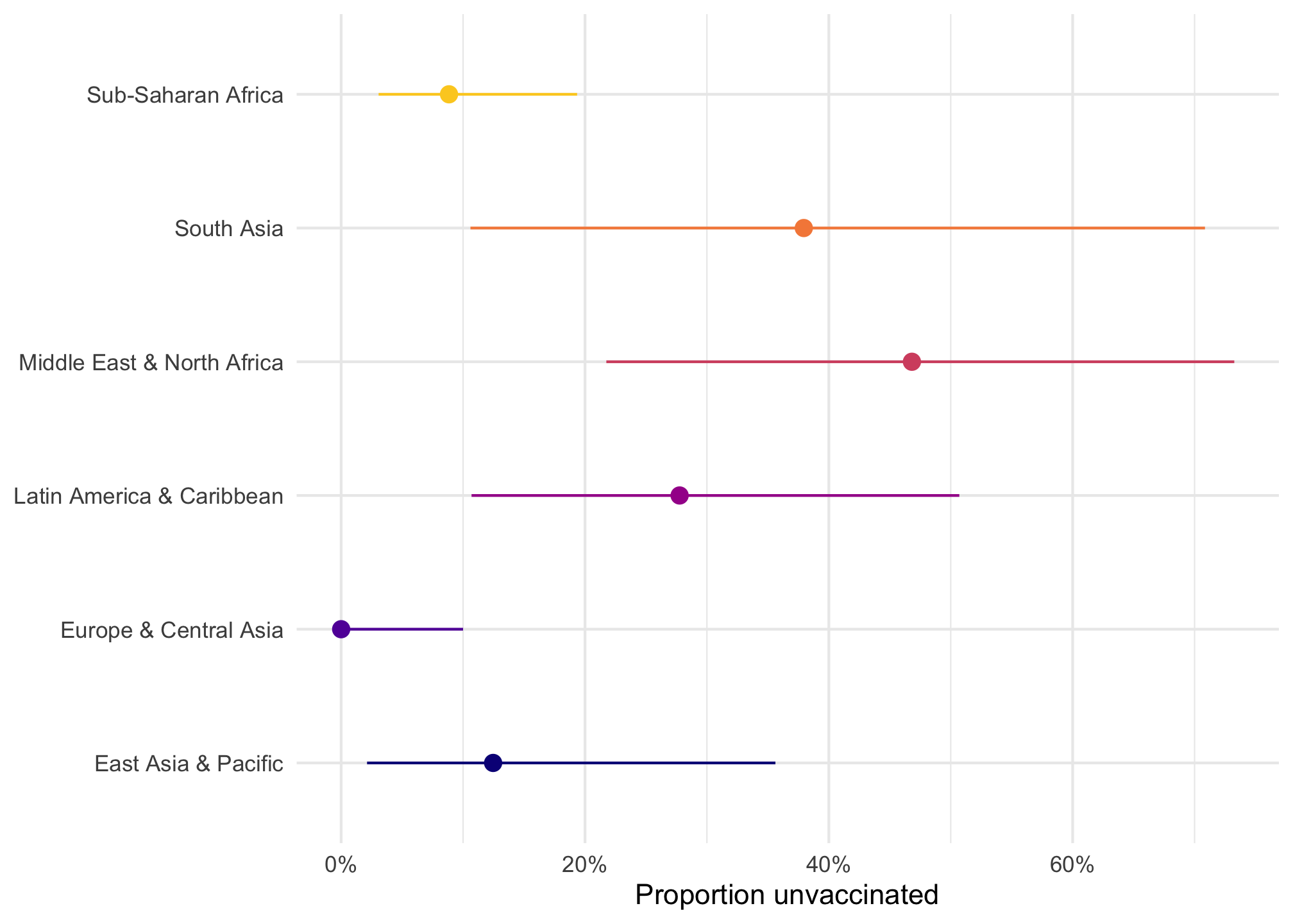
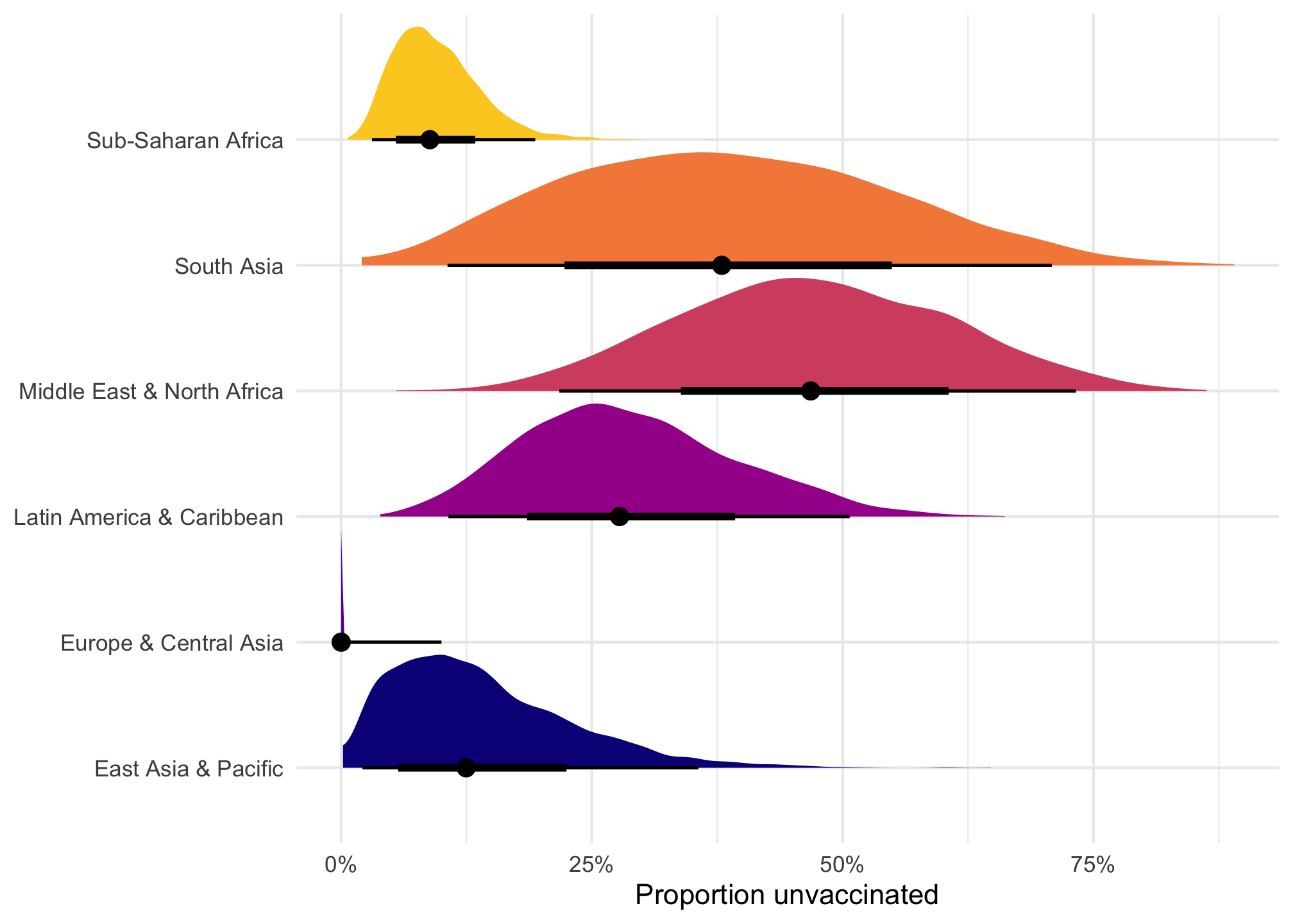
We can look at the individual parts of this model. Here are the posterior predictions of 0s across each region:
Code
# With {marginaleffects}model_beta_zi |>plot_predictions(condition =c("region", "region"), dpar ="zi") +scale_y_continuous(labels =label_percent()) +labs(x =NULL, y ="Proportion unvaccinated") +scale_color_viridis_d(option ="plasma", end =0.9, guide ="none") +coord_flip()
Code
# With {tidybayes}model_beta_zi |>linpred_draws(newdata =data.frame(gdp_per_cap =10000, region =unique(tetanus_2020$region)),dpar ="zi", transform =TRUE ) |>ggplot(aes(y = region, x = zi)) +stat_halfeye(aes(fill = region), normalize ="xy") +scale_fill_viridis_d(option ="plasma", end =0.9, guide ="none") +scale_x_continuous(labels =label_percent()) +labs(y =NULL, x ="Proportion unvaccinated")
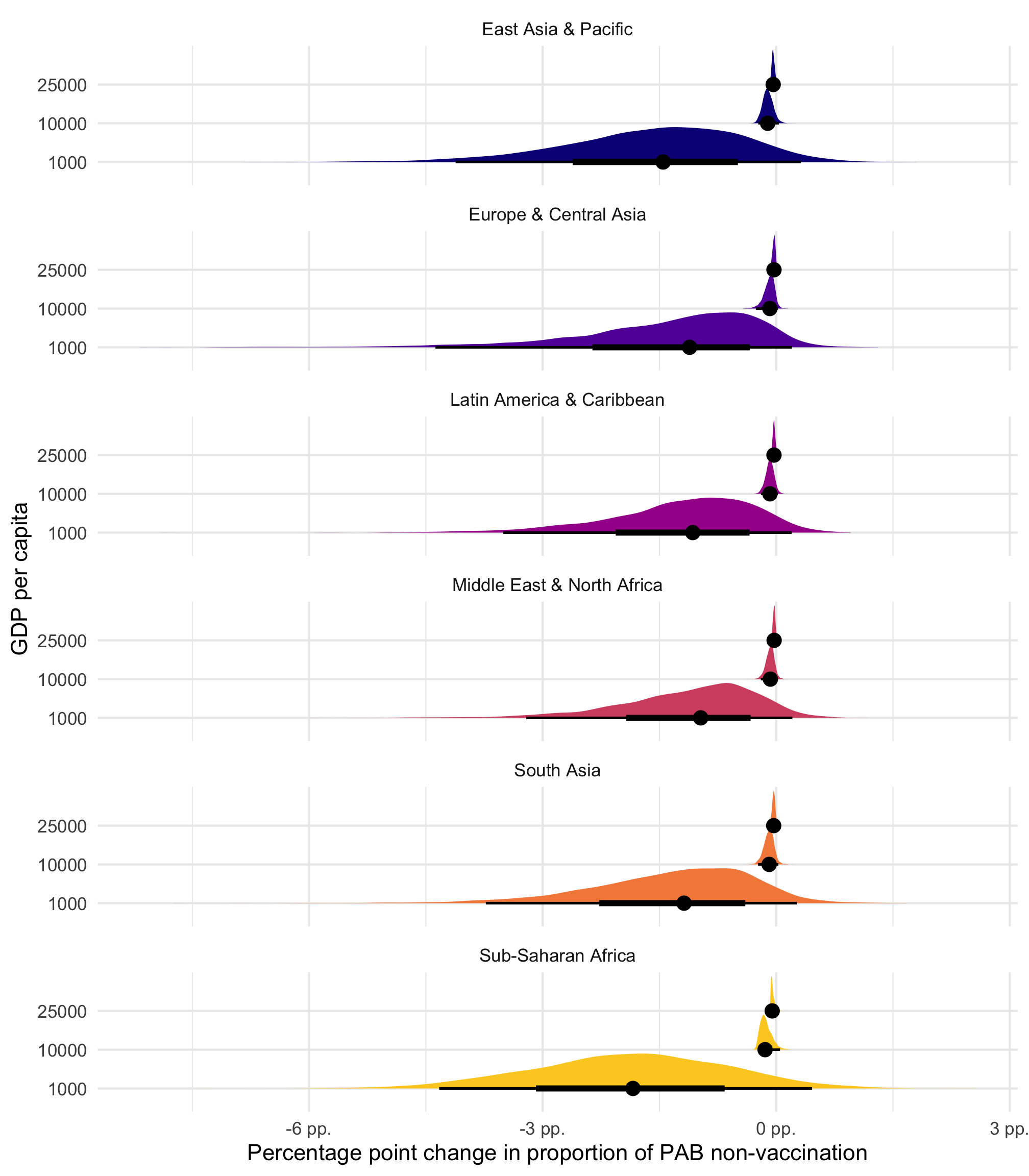
All the regular {marginaleffects} and {tidybayes} functions work too, either on individual parts of the model (with the dpar argument), or on both combined (without any extra arguments). Like this—we can visualize the posterior distributions of the specific marginal effects while also incorporating the 0 process!:
Code
model_beta_zi |>slopes(newdata =datagrid(gdp_per_cap =c(1000, 10000, 25000), region = unique),variables ="gdp_per_cap" ) |>posterior_draws() |>mutate(draw = draw *1000) |>ggplot(aes(x = draw, y =factor(gdp_per_cap), fill = region)) +stat_halfeye(normalize ="xy") +scale_x_continuous(labels =label_number(scale =100, suffix =" pp.")) +scale_fill_viridis_d(option ="plasma", end =0.9, guide ="none") +facet_wrap(vars(region), ncol =1) +labs(x ="Percentage point change in proportion of PAB non-vaccination", y ="GDP per capita" )